Purchasing a Home versus Renting and Investing

​Buying a home is typically the largest investment a household makes. One alternative is to rent a home and invest any savings from renting in something else. From purely an investment perspective, the anticipated rate of return plays a crucial role in the homebuying decision. This report compares the financial gains from renting and investing any remaining cash in the stock market with the gains from purchasing a home. Households faced with such a choice should consider the historic performance of both before making their choice.

The point of initial investment ranges from the beginning of 2000 to the beginning of 2016, a period with significant disruptions in both the stock and housing markets.

Multiple investment opportunities are available to households. However, stocks and real estate have shown to be two of the more popular. According to the Survey of Consumer Finances (conducted by the Federal Reserve Bank), 63.7 percent of all families in the United States held a primary residence in 2016, while 51.9 percent of all families had direct or indirect stock holdings.

Although the proportion of families who held a primary residence was somewhat similar to the proportion of families with direct or indirect stock holdings, the values of the assets differed significantly. In 2016, the median value of stocks for families with direct or indirect stock holdings was $40,000, whereas the median home value was almost five times that at $185,000. Note, however, that the amount of actual home equity is affected by any remaining mortgage balance, assuming the home is mortgaged at all.

By renting and investing in a stock portfolio, the household forgoes the potential to earn appreciation from homeownership but may benefit from selling the stock at a profit. Conversely, by purchasing a home, the household forgoes the future earnings from a stock portfolio as well as the potential to earn dividends. Renting can cost more than homeownership, in which case a renter household might not be able to invest any excess funds in a stock portfolio.

The question is, if between 2000 and 2016 a Texas household had the option of either renting (and consequently investing in the stock market) or purchasing a home, which provided the greater financial gain? The answer isn’t simple.

Scenario 1: Stocks ve​rsus Homes

Numerous differences complicate a comparison between renting and investing in the stock market and purchasing a home. The Real Estate Center’s analysis attempted to control for the differences through a number of initial assumptions in this first scenario. (The assumptions are expanded in a second, more complex scenario later in this report.)

• The household either purchases a home or rents and invests the entire down payment in a stock portfolio at the beginning of the year.
• In the case of a home purchase, the household meets the qualifying requirements for purchasing a home. 
• In the case of an investment in stocks, the household does not trade any stocks during the holding period and reinvests all dividends (a buy-and-hold investment strategy).
• The household does not face any constraints in the sale of either the stock portfolio or the home.
• The internal rate of return (IRR) results are the sole criteria for buying versus renting (see “Using IRR as a Benchmark"). The analysis does not account for qualitative differences between owning and renting.
• Households seek a longer-term investment in a primary residence. Second home or investment property purchases are not considered.

Under this first scenario, assume a household with $10,000 has two options: rent and open an investment portfolio or spend the money on a down payment on a home. For this initial analysis, the home price is assumed to be $100,000, resulting in a loan-to-value (LTV) ratio of 90 percent.

Investme​​​​nt Portfolio

The value of the investment portfolio at the end of each year, after a minimum two-year hold, depends on the year the $10,000 was invested (Table 1). Table 2 depicts the IRR on the initial investment based on the year in which the portfolio is liquidated.

The timing of the initial investment, the duration of the holding period, and the volatility in the stock market during the holding period produce dramatically different returns. In general, opening a portfolio in a year with strong stock market returns produces a higher initial IRR due to the positive impact of compounding in the early years.

For example, a portfolio opened in the beginning of 2003 earned an average IRR of +12.7 percent after five years (at the end of 2007). The high return stems from the large initial upswing in the market in the first two years (+19.2 percent) as well as strong average IRRs across the later holding periods, ranging from +12.7 to +14.6 percent (Table 2). Higher growth in the initial years of a holding period effectively acts as a hedge against future market downturns.

Conversely, a portfolio opened in a year characterized by a stock market decline needs much higher growth in subsequent years to recoup the early losses during the initial years of the holding period. A stock portfolio opened in the beginning of 2002 earned an IRR of just +6.1 percent after five years (at the end of 2006). Return is significantly lower, as the average +0.1 percent IRR over 2002 and 2003 lessened the impact of subsequent stock market growth on the portfolio’s value (Table 2).

How do the returns compare if both portfolios were sold at the end of 2008 during the early stages of the Great Recession (GR)? At +2.4 percent, the average IRR for a portfolio opened in 2003 remains slightly higher than the –1.5 percent IRR for a portfolio opened in 2002. The poor +0.1 percent average IRR over 2002 and 2003 diminished the ability of the portfolio opened in 2002 to offset the downturn in 2008. By comparison, the initial strong growth of +19.2 over 2003 and 2004 allowed the portfolio opened in 2003 to better offset the decline from the recession that began in 2008 (Table 2).

​

Home P​​urchase

Home values at the end of each year the home could have been sold, based on the year of purchase and Federal Housing Finance Agency (FHFA) home price appreciation data for Texas, are shown in Table 3. Table 4 shows the IRR based on those values.

Similar to renting and investing in the stock market, the return for a home purchase is affected by the timing of the initial investment and the duration of the holding period. While high market volatility significantly impacted the range of stock market investment returns, the low volatility in Texas’ housing market tempered homeowners’ returns.

Overall, lower volatility translated into much less IRR variation from homeownership than from the S&P 500 portfolio. Annual IRR ranged from –1.3 to +7.9 percent for a home purchase (Table 4) versus –18.2 to +23.8 percent for the stock market portfolio (Table 2). Thus, households had the potential to earn a significantly higher rate of return from the stock market than from owning a home. However, they also risked losing substantially more money. Both results rely heavily on the timing of the initial investment.

In the years immediately preceding the GR’s housing downturn, the return on homeownership remained relatively unchanged. Unlike states such as California and Florida, Texas experienced neither excessively high home price appreciation during the national housing boom of the mid-2000s nor the exceptional price decline immediately after the GR.

Since the GR, Texas home prices have increased more rapidly. For homes purchased from 2013 to 2016, the IRR from homeownership ranged from +5.9 to +7.9 percent (Table 4).

More Reward​ing Investment?

Based on IRR, renting and investing in the stock market was generally the more financially rewarding option for a household between 2000 and 2016 in this first scenario (Table 5).

If the initial investment was made in 2000 or 2001, homeownership was, on average, the option that yielded a higher return through 2012. However, for all other years, on average, renting and investing in the stock market proved the more financially beneficial option.

Alternatively, the higher incidence of negative returns and greater return volatility experienced in the stock market indicates renters assumed much greater risk compared with buying a home. The IRR from a stock portfolio produced negative returns 23 times (Table 2). Meanwhile, IRR from homeownership produced negative returns in only six instances (Table 4).

Furthermore, the severity of the negative returns was much greater for an investment portfolio than for homeownership (–18.2 percent versus –1.3 percent). On average, the potential loss in initial investment proved higher for renters than for homeowners. The IRR from the stock portfolio varied significantly across holding periods, whereas the IRR from homeownership remained in the low single digits.

Note that the analysis for renters who chose to invest in the stock market portfolio reflects before-tax returns. Capital gains tax is not factored into the returns for the stock market or homeownership in this first scenario.

According to the Tax Policy Center, the average effective tax rate for capital gains ranged from a low of 12.5 percent in 2009 to a high of 19 percent in 2000. This represents a significant portion of the overall value of the stock portfolio and would have a large impact on its after-tax return.

Weighing th​​e Options

On average, renting and investing in the stock market offered a greater IRR than purchasing a home for Texas households from 2000 to 2017 under this first set of assumptions. However, the introduction of capital gains tax can affect the investment decision. Under current tax law, avoiding capital gains tax on sale of a home gives homeownership a tremendous edge. The impact of both capital gains tax and transaction costs is introduced in a second scenario.

Scenario 2: A More “Re​​al-World" Comparison

This scenario considers the IRR from homeownership across four major Texas MSAs along with the State of Texas. The four metros discussed are Austin, Dallas-Fort Worth, Houston, and San Antonio.

Like Scenario 1, Scenario 2 compares the IRR from homeownership to that from renting and investing in the stock market. However, it also considers expenses associated with buying, holding, and selling a home or a stock portfolio in a typical, real-world situation. The amount of the initial investment varies, but it is assumed to be the same for both investment options.

Home Purchase Ass​​umptions

A few assumptions are changed for this second scenario.

• The sum of the down payment on a home plus the closing costs represents the initial investment. The down payment for a home purchase is 20 percent.
• The dollar amount available to either purchase or rent varies by the five geographies and year of investment due to changes in median home prices.
• According to the U.S. Census Bureau, 58 percent of the total owner-occupied housing units in Texas were mortgaged in 2016. This analysis assumes households require a mortgage and must pay principal and interest.
• Homeowners must also pay property taxes, insurance, and maintenance costs.
• Both homeowners and renters pay for utilities separately. Therefore, utilities are a wash, and this analysis does not consider them.
• Because this analysis assumes a minimum two-year holding period for a principal residence, no capital gains tax on a sale by homeowners is factored in.
• A 30-year, fixed-rate mortgage at the effective mortgage interest rate was calculated for each geography. However, mortgage interest rates vary slightly by Metropolitan Statistical Area (MSA). For the state, the rate ranged from a low of 3.75 percent in 2012 to a high of 8.16 percent in 2000. FHFA is the source for mortgage interest rate data.
• Closing costs are 2 percent of the purchase price.
• Selling fees are 6 percent of the sales price.
• Property taxes are pegged at 2 percent of the home value while insurance and maintenance costs are 1.5 percent.
• Homeowner net cash flows equal the outflow of mortgage principal and interest, property taxes, and insurance and maintenance plus the inflow of rent on a “comparable" property.

These additional assumptions are intended to represent reasonable estimates of actual market conditions. Different loan terms or expenses associated with homeownership can alter the return on homeownership and potentially reverse the investment decision.

Renter Stock Portfolio ​Assumptions

Stock portfolio expenses paid by renters typically include purchase and sale broker commissions (i.e., transaction fees) as well as capital gains tax on the sale of individual stocks or the portfolio itself. Assumptions for this scenario:

• As in Scenario 1, the renter household does not make any transactions over the holding period of the investment portfolio.
• As stock transaction fees are generally quite low (1 percent or less), they are excluded from the analysis.
• Scenario 2 factors in capital gains tax on a stock portfolio, with the rate being 12.5 to 19 percent of the overall value of the portfolio, depending on tax law at the time.
• Since a renter household does not make any transactions over the holding period of the portfolio, the tax is applied to the value of the stock portfolio only when it’s liquidated—as long as the portfolio realizes a gain in value. 
• If the portfolio loses value over its holding period, renter households are not subject to capital gains tax on the sale of the portfolio.

Rental P​​roperty Assumptions

For households choosing to rent and invest in the stock portfolio, the following assumptions apply:

• Monthly rent is the sole cash outflow for renters. No utilities are considered.
• The rental property is comparable in quality and functionality to one a homeowner would purchase.
• Annual cash inflows to renters are the annual expenses associated with homeownership offset by the difference between owning and renting.
• A household that rents and decides to open a stock portfolio reinvests the difference between owning and renting. (Actual renters often lack the discipline to actually deposit such funds into a stock portfolio each month. This study assumes a disciplined investor.)

No rental rate index for the five specific geographies was available. Therefore, annual rents were calculated by adjusting the 2015 median rent for each geography reported in the American Community Survey by the annual consumer price index reported by the U.S. Bureau of Labor Statistics.

Cash-Flo​​w Fluctuations

Net cash flow to homeowners is typically negative, as the annual costs of homeownership usually outweigh the rent on a “comparable" property. However, upward pressure on rents has translated into positive cash flows for homeownership over the past several years.

Rental rates in some Texas metros have been also quite volatile. For example, from 2000 to 2017 Dallas-Fort Worth rent growth ranged from -2.9 percent to +7.0 percent, averaging +3.1 percent each year. Meanwhile, the annual cash outflows associated with homeownership in DFW increased, on average, 1.6 percent each year.

Purchasing a home in 2016 in DFW would have resulted in a negative cash flow for the first year (-$264.48) but a positive cash flow for the second year (+$141.30), as annual average rent exceeded the annual average costs of homeownership. In essence, rent growth outpaced the growth in homeownership costs between 2016 and 2017.

Homeownership costs tended to remain more stable than rental rates over the holding periods, as the sum of principal and interest is constant for a fixed-rate mortgage. Property taxes and insurance and maintenance can vary each year depending on factors such as the appraised value of the home. However, the sum of these expenses was generally less than the sum of mortgage principal and interest, thus having less impact on overall homeownership costs.

Scena​​rio 2 Results

Even if a household suffered an overall financial loss from a particular investment (as indicated by a negative IRR), the investment with the less negative IRR is assumed to provide the household with greater financial gain. In other words, a superior IRR does not necessarily translate into a positive IRR.

The results for the investment decision (i.e., the number of times a household most often captured a higher IRR from purchasing a home or renting and investing in the stock market during the study period) vary by geography. However, the IRRs from homeownership exceeded the IRRs from renters investing in the stock market in all five MSAs and Texas overall.

The Winnin​​​g IRR Tally

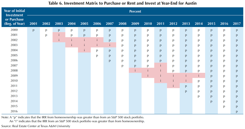
Of the four major MSAs, Austin had the most occurrences of an IRR that was greater for homeownership. Over the study’s 153 individual holding periods, the IRR for homeownership exceeded that from renters investing in the stock market 130 times, or 85 percent of the time (Table 6).

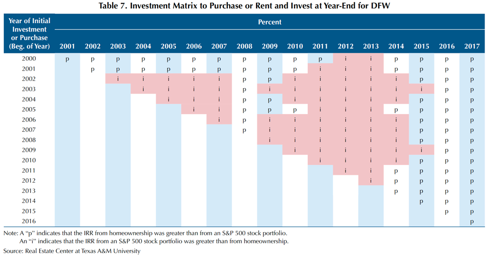
In DFW, the IRR from homeownership surpassed that of renters investing in the stock market 82 times, or 53.6 percent of the time (Table 7). In Houston, the frequency was 121 times, or 79.1 percent (Table 8), and in San Antonio, 113 times, or 73.9 percent (Table 9).

​

Results using statewide median home price appreciation are in Tables 10 and 11. The IRR from homeownership in Texas surpassed that of renters investing in the stock market 97 times, or 63.4 percent of the time, suggesting that home price increases in the state’s four major metros have generally been stronger than in less urban areas.

Incidence of Posit​​​ive versus Negative IRRs

The results also indicate that either renting and investing in the stock market or buying a home would have produced more positive than negative returns. However, homeownership did result in a greater incidence of positive returns in every case.

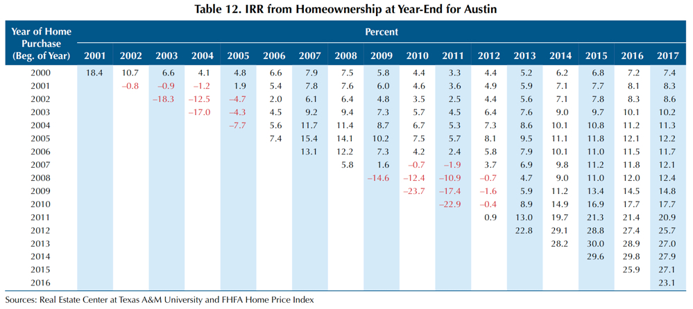
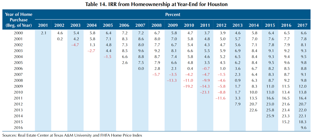
In Austin, the IRR from homeownership was positive in 133 instances, or 86.9 percent of the time (Table 12). DFW had 116 occasions, or 75.8 percent (Table 13); Houston 134, or 80 percent (Table 14); and San Antonio 127, or 83 percent (Table 15). Statewide, the homeownership IRR was positive 126 times, or 82.4 percent of the time (Table 10).

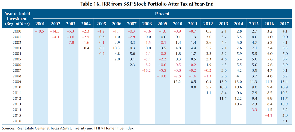
The IRR from renters investing in the stock market was the same regardless of geography, with a positive IRR occurring in 113 instances, or 73.9 percent of the time (Table 16).

When Rent​​ing and Inv​​​esting in Stock Market Paid Off

In Austin, the instances in which renters investing in the stock market provided a superior IRR to purchasing a home are characterized by a shorter investment horizon (between one and five years). For example, a household that invested in the beginning of 2003 would have witnessed greater financial gain by renting and investing in the stock market if the household had disinvested in the first four holding periods (at the end of 2004, 2005, 2006, and 2007) (Table 6).

For households that invested from 2011 onward and disinvested from 2013 to 2017, the return on homeownership measured significantly higher than the return on a renter’s investment portfolio (Table 6). This is largely a result of substantially higher returns on homeownership within that period compared with previous periods.

From 2000 to 2017, homeownership in DFW provided, on average, only slightly greater financial gain than renters investing in the stock market. Compared with the other three major metros and the state, DFW homeownership returned the fewest incidences of superior IRR (Table 7).

Renters investing in the stock market produced a higher IRR for a household making the initial investment between 2002 and 2004 or between 2006 and 2010. Irrespective of the year of initial investment, investing in the stock market generally provided greater financial gain for a household that disinvested between 2005 and 2007 or between 2010 and 2014. However, disinvestment since 2015 would have resulted in homeownership providing the superior IRR.

The disparity in IRR between renters investing in the stock market and buying a home in the DFW market has widened significantly in the last several years. For a household choosing the home purchase option in 2014 through 2016, the IRR would have ranged between +25.1 percent and +32.0 percent (Table 13).

Overall, from 2000 to 2017 homeownership in Houston proved more financially beneficial than renting and investing in the stock market (Table 8). However, on average, renters investing in the stock market did provide a superior IRR to purchasing a home for households that invested from 2008 to 2010.

Houston homeownership consistently posted double-digit returns for households that invested between 2013 and 2015. For a household that invested in 2014, the IRR from homeownership would have been +25.9 percent, +23.3 percent, or +22.1 percent, depending on year of disinvestment (Table 14).

Similar to Houston, from 2000 to 2017 San Antonio homeownership produced, on average, greater financial gain than renters investing in the stock market. However, the stock market did provide a superior IRR to renters investing from 2008 to 2010 (Table 9).

Regardless of the year of initial investment, the IRR on homeownership overwhelmingly outpaced that of the stock market for households that disinvested from 2015 to 2017 (Table 9). The larger disparity in the IRR between investment options is a factor of both home price appreciation and growth in rent above the costs of homeownership.

Across Texas, from 2000 to 2017 homeownership yielded an IRR superior to renters investing in the stock market. Furthermore, above-average home price appreciation from 2013 to 2015 facilitated significantly higher returns from homeownership (Table 11).

Overall Conclusions

Scenarios 1 and 2 yield vastly different results. Scenario 1 found that renting and investing in the stock market was, on average, the option that offered a greater IRR for households in Texas from 2000 to 2017. Conversely, using home price appreciation from the four major Texas MSAs as well as the state, Scenario 2 revealed that purchasing a home generally provided households with a superior IRR.

A major factor in the different outcomes between scenarios was the effect of capital gains tax on a renter’s investment portfolio. The introduction of capital gains tax in Scenario 2 dramatically impacted the IRR from an investment portfolio. In most cases under current tax law, avoiding paying capital gains tax on the sale of a home gives homeownership a tremendous edge.

Additionally, high rent growth over the past several years has diminished the financial gain from investing any excess funds in the stock market. Across the four major MSAs, rent on a “comparable" property typically outweighed the annual costs of homeownership by the end of any given holding period.

An important factor to consider is the substantial up-front cost of purchasing a home versus renting and investing in the stock market. Potential homeowners should typically expect to remain in a home at least two years before the front-end costs are recouped.

Finally, renters investing in the stock market at the end of a recession and disinvesting within a few years almost always captured the superior financial investment. The stock market tends to grow at a much faster rate than home prices coming out of a recession. However, over longer time periods purchasing a home has shown to be the winner.

Ultimately, a household’s decision to rent and invest in the stock market or purchase a home will be determined by a combination of these and other factors. This analysis considered only the IRR a household would have received from either investment option.

Likewise, a household’s decision to rent and invest in the stock market or purchase a home will be determined by a combination of personal and investment preferences, not just the IRR the household would have received from either option. Households are likely to consider factors such as each market’s historic performance and its current conditions, and the ease and ability of qualifying for homeownership.

Other factors include the need for flexibility in living arrangements, the obligations of homeownership, available housing stock, nearby amenities, and the social and community aspects of owning versus renting.

_______________

Dr. Hunt ([email protected]) is a research economist and Losey a research intern with the Real Estate Center at Texas A&M University.